

Our article series on Autonomous Exploration for Mobile Robots is back! For this third episode, the Awabot Intelligence team dissects frontier-based exploration, which has established itself as the benchmark method following the comparison published in the previous article.
Principle of autonomous frontier-based exploration
As a reminder, this method implies that the mobile robotic solution explores the environment by continuously moving towards new frontiers.
What are occupation grid and frontiers ?
To understand the frontiers-based algorithm, one must first define two concepts: the occupation grid and frontiers.
An occupancy grid is one way of representing the environment. It breaks down space into a set of cells of the same size. These cells store an occupancy probability that can be used to determine whether the space corresponding to each cell is free, occupied, or unknown.


- A list of adjacent free cells;
- A size: the number of cells contained in a frontier;
- A distance: the Euclidean distance, which corresponds to the shortest distance, between the robot and the frontier (in meters);
- An orientation: the angle between the direction of the robot and the candidate frontier (in degrees);
- A centroid: the point at the center of the masses of the frontier;
- A cost: the cost calculates the interest of a frontier to be visited.
How does the robot choose the next frontier?
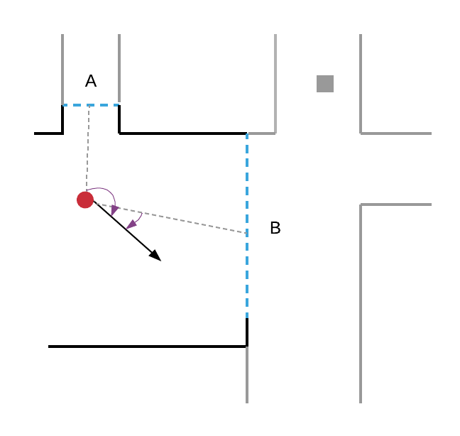
Suppose a mobile robot in an unknown environment detects two frontiers A and B. How does the robot choose the next frontier to visit?

Example of frontiers detected by a robot
The principle is simple: the robot will simply choose the frontier which has the lowest cost among the candidate frontiers.
In our study, the concept of cost is established according to the following function:
C(ƒ) = λ1Distance(ƒ) – λ2Size(ƒ) + λ3Orientation(ƒ) (1)
[Gao et al., 2004]
With :
- ƒ : a frontier of F
- λ1, λ2 et λ3 : weight parameters normalized between 0 and 1
According to equation(1), an interesting frontier to visit, that is to say with a relatively low cost, is a frontier close to the robot, large in size and facing it.
The goal is for the robot to explore an entire environment in a minimum of time and using as few resources as possible:
- if a frontier is close, the robot will access it in less time and using fewer resources;
- if a frontier is large, then there is a good chance that a large unexplored area of substantial size lies beyond it. We will therefore acquire more information on the environment ;
- if a border is in front of the robot, this prevents it from wasting time turning around to find its way.
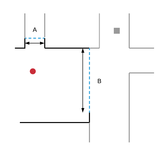
In order to illustrate these concepts, the diagrams (a), (b) and (c) below break down the frontiers according to the three criteria of distance, size and orientation. In particular, we observe that the frontier A is closer to the robot than the frontier B, but smaller and with a higher angle with respect to the robot.
To find a compromise between distance, size and orientation, we use weight parameters λ1, λ2 et λ3: putting more weight on one of the factors allows it to be prioritized. In our study, these values were fixed thanks to various tests (i.e., gridsearch).
 Distance")
 Orientation")
 Size")
Autonomous frontier-based exploration: presentation of the algorithm
The first step is to detect frontiers using the robot’s sensors (LiDAR sensor in our case). The algorithm scans the occupancy grid and identifies all free cells adjacent to unknown cells, resulting in candidate boundaries. Among these candidate frontiers, it selects the one with the lowest cost according to equation (1) and recovers its centroid point which becomes the new destination of the robot (algorithm 1).
Algorithm 1: Exploration of frontiers
1: G ← Occupancy grid
2: Do
3: F = DetectBorder (G)
4: D = SelectBorder (F)
5: While F is not empty
6: End While
The boundary exploration algorithm is repeated every second. Periodically, the robot detects new frontiers from the constructed occupancy grid and selects a new destination to reach to obtain new information about its environment. The algorithm ends when the robot no longer detects a new frontier, that is, when all of the space is assumed to be known.
Autonomous frontier-based exploration
Implementation
This solution was implemented on the Turtlebot3 Burger robot thanks to the Robot Operating System (ROS) middleware and the Gazebo software which makes it possible to simulate the robot and the environments.
Would you like to know more about the tests and results obtained by this autonomous exploration solution? See you next month!

